You ran a retirement simulation and got two numbers. The historical backtest says 98.9% success. The Monte Carlo says 90.5%.
Which one is right? Both — but they're doing different things. Here's what each one actually calculates.
What Monte Carlo Simulation Does
Monte Carlo generates thousands of synthetic return sequences by drawing from a statistical model. Each year's return is sampled independently — a random draw from a calibrated distribution.
This gives you a probability statement: "Given our model of how markets behave, there is an 90.5% chance your portfolio survives 30 years."
The strength is coverage. Monte Carlo can generate scenarios that haven't happened yet — combinations of inflation, returns, and timing that are statistically plausible but absent from the historical record. It stress-tests your plan against a wider range of possible futures than history alone provides.
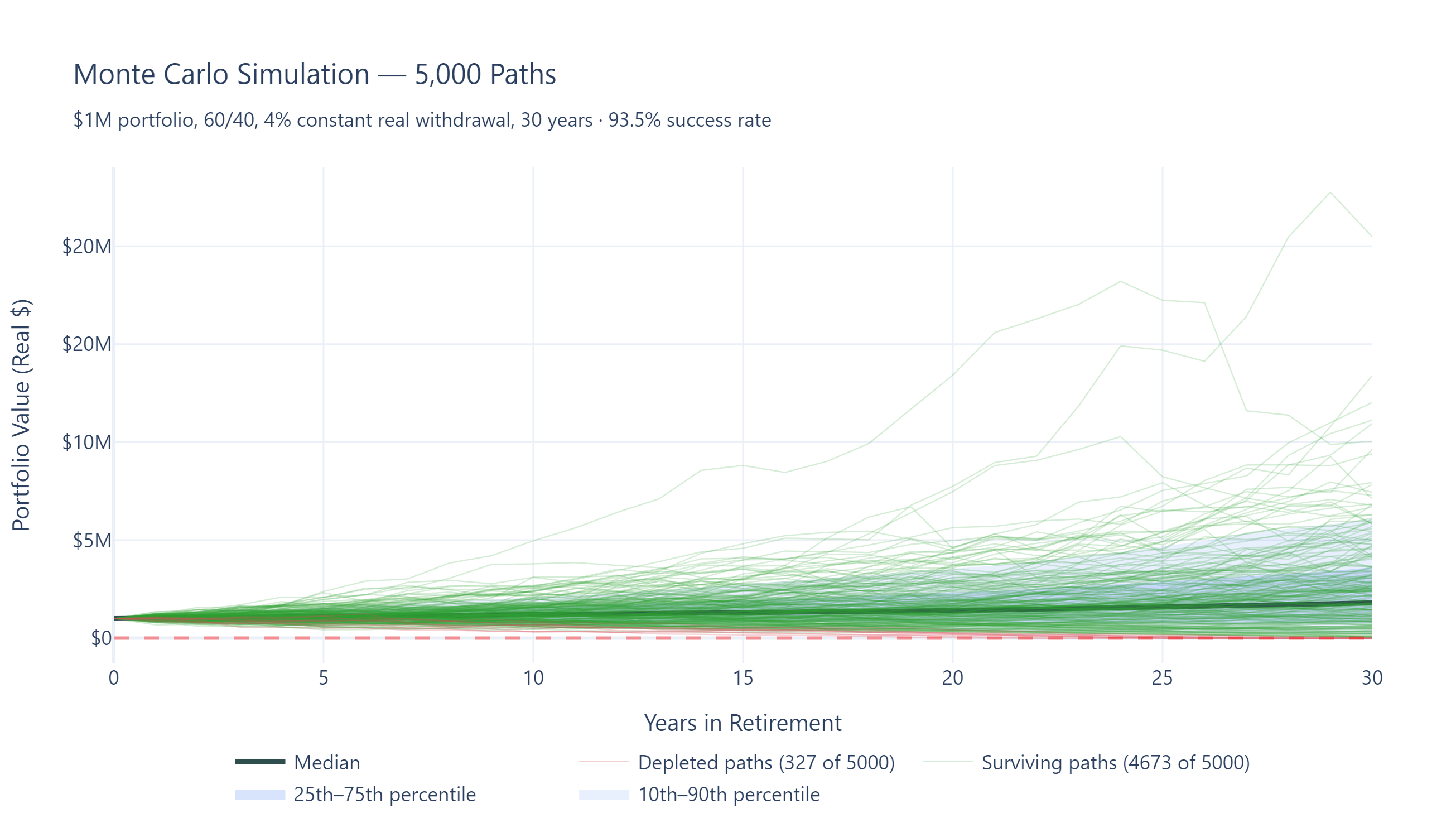
Monte Carlo fan chart — 5,000 simulated portfolio paths. The wide spread reflects the full range of outcomes the model considers possible, including sequences history never produced.
The Independence Assumption
There is a well-known limitation here. Each year's return is drawn as if markets have no memory. In reality, markets exhibit momentum, mean reversion, and regime clustering. A bad year raises the odds of recovery. A great decade raises the odds of a correction.
Monte Carlo doesn't know this. It treats every year as a fresh coin flip. It can produce sequences — eight terrible years followed by eight more with no reversion — that are statistically possible but historically rare.
The independence (iid) assumption is the most common critique of Monte Carlo in retirement planning. More complex models exist — regime-switching, GARCH, block bootstrap — but each introduces its own calibration choices. You trade a simple, understood bias for a more opaque one.
What the Research Shows
This isn't just a theoretical concern. Derek Tharp, writing on Kitces.com, tested this directly: a withdrawal rate that succeeded in 100% of historical rolling periods only achieved a 93.5% success rate in traditional Monte Carlo. That 6.5% gap is entirely manufactured by the model — those failing scenarios are worse than anything that has ever actually happened.
The culprit isn't fat tails. Using Shapiro-Wilk testing on data from 1871 onward, Tharp found that annual 60/40 portfolio returns show no statistically significant deviation from a normal distribution. Daily and monthly returns have fat tails; annual returns do not. The real issue is negative serial correlation — bear markets tend to precede bull markets as valuations reset. Standard Monte Carlo ignores this entirely, projecting unnecessarily volatile long-term sequences.
The worst Monte Carlo scenario in Tharp's analysis exhausted funds after just 15 years. The actual worst historical scenario — the 1966 retiree — lasted the full 30 years (this may vary slightly depending on assumptions). Over 6% of Monte Carlo outcomes were worse than anything the real world has ever produced.
What Historical Simulation Does
Historical simulation takes every real rolling period from the available data — every 30-year retirement starting from 1871, from 1872, and so on — and runs your plan against each one.
This gives you an enumeration: "Your portfolio survived in 114 out of 120 tested scenarios."
There is no probability model. No distributional assumption. No parameters to calibrate. Just: here is what actually happened, and here is how your plan would have fared in each case.
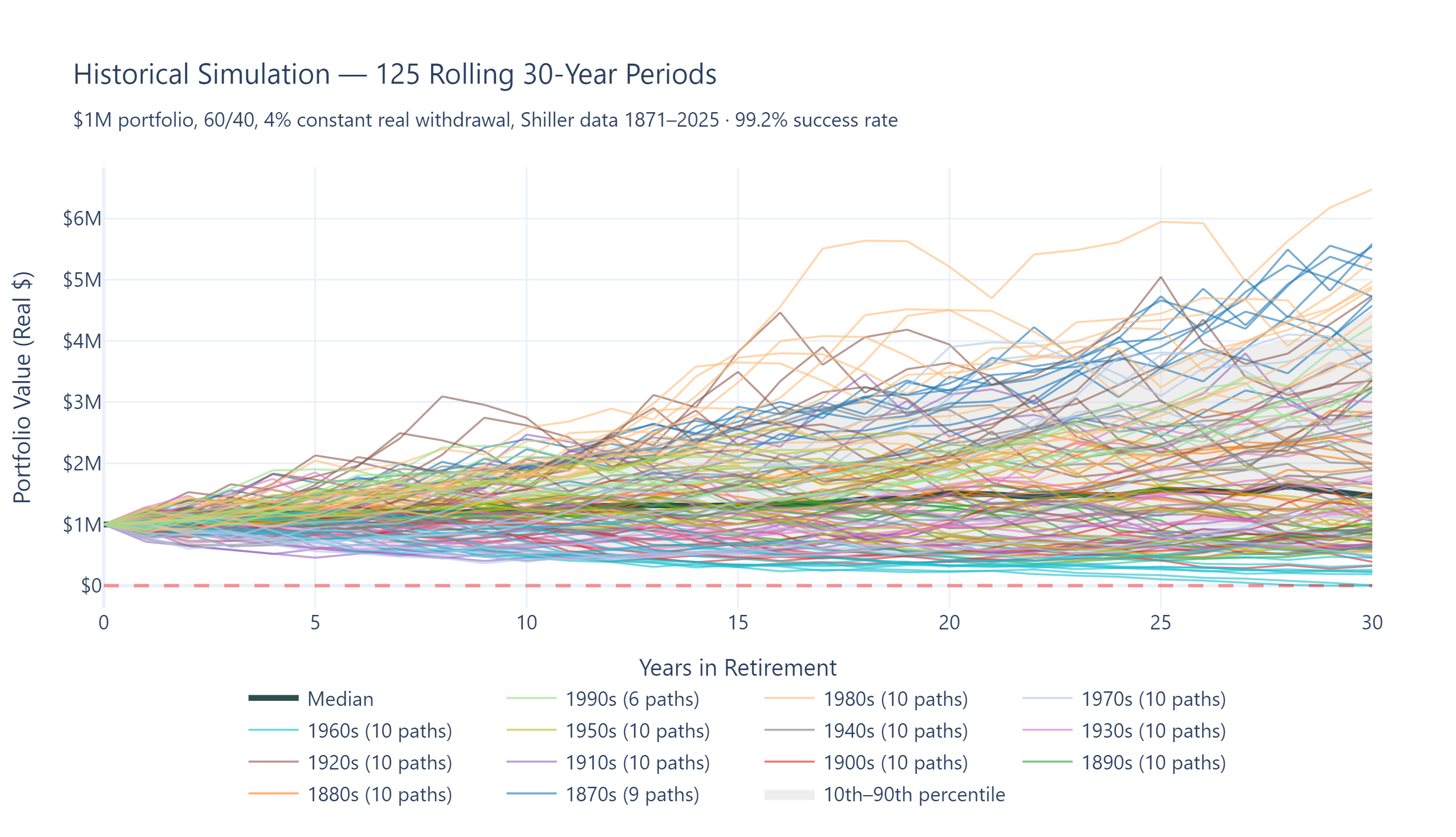
Historical portfolio paths — every real 30-year retirement cohort since 1871. Each line is a sequence that actually happened, with real serial correlations, real crashes, and real recoveries.
The strength is realism. Every scenario is a real sequence with real momentum, real regime transitions, real recoveries following real crashes. The 1973–74 bear market is followed by the actual recovery that happened — not a random draw that might or might not recover.
The limitation is coverage. You only have the scenarios history gave you. There may be plausible futures that have no historical precedent.
How Well Do They Predict?
In 2023, Tharp and Fitzpatrick measured this directly, testing how well different simulation approaches predict real-world retirement outcomes using Brier Scores — a standard metric for forecast accuracy where lower is better.
The results were clear: Historical simulation and Regime-Based Monte Carlo outperformed Traditional Monte Carlo by about 25% on predictive accuracy. Real market data captures dynamics like momentum and mean reversion that conventional Monte Carlo discards.
Most people assume Monte Carlo is "the conservative one." Tharp and Fitzpatrick's research shows it's more accurate to say Monte Carlo is differently wrong — it overstates some risks, understates others, and reshapes the relationship between withdrawal rate and success probability in ways that don't match how markets have actually behaved. As the crossover pattern below illustrates, at higher withdrawal rates Monte Carlo can actually be more optimistic than the historical record.
The Gap Between Them
Monte Carlo results depend on the exact distributional assumption we make. We may try to fit different return distributions to the same data. Each of these will lead to somewhat different results. However, we can make the following observations that seem to hold in general. At low withdrawal rates, Monte Carlo tends to produce lower success rates than historical backtesting — the conservatism gap most people expect. But that pattern reverses at higher withdrawal rates.
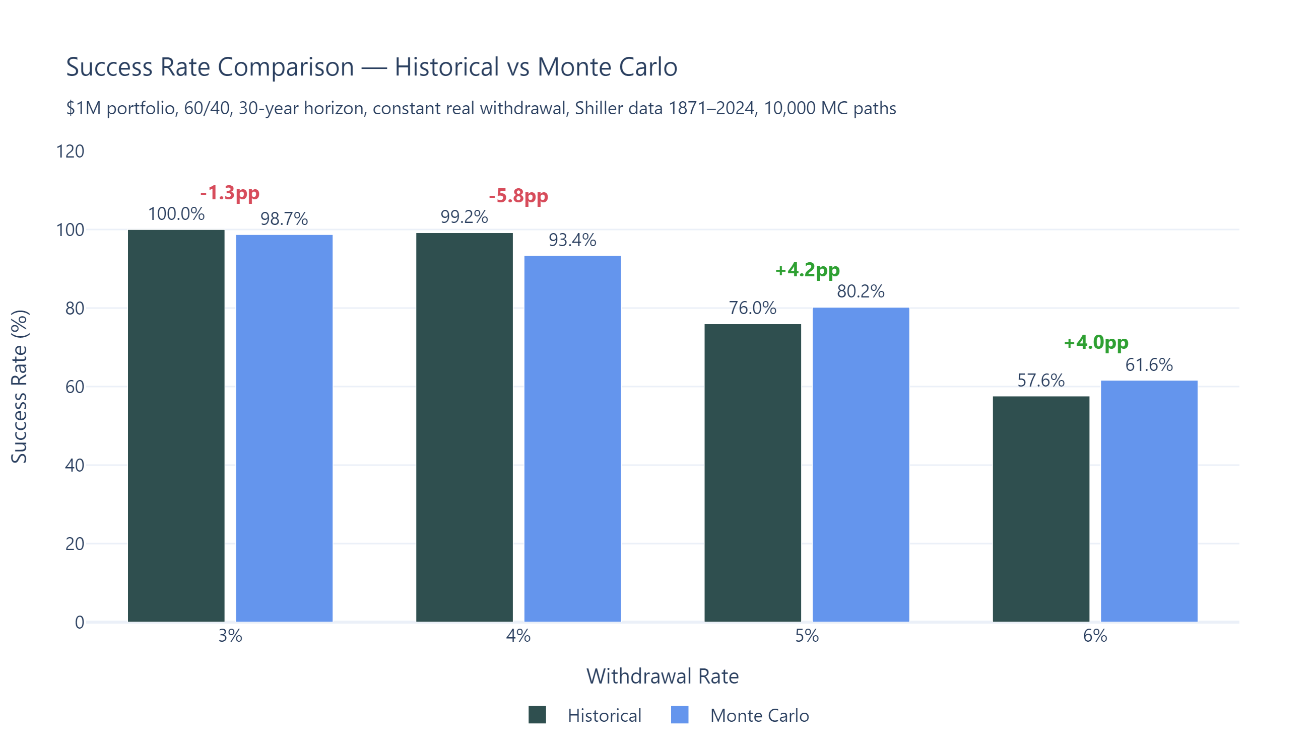
Success rates compared — Monte Carlo vs Historical across withdrawal rates (3% to 6%), 60/40 portfolio, 30-year horizon. Note the crossover: MC is more conservative at low rates but more optimistic at high rates.
| Withdrawal Rate | Historical Success | Monte Carlo Success | Gap |
|---|---|---|---|
| 3.0% | 100.0% | 98.7% | -1.3pp |
| 4.0% | 99.2% | 93.4% | -5.8pp |
| 5.0% | 76.0% | 80.2% | +4.2pp |
| 6.0% | 57.6% | 61.6% | +4.0pp |
Bellavia simulation results — $1M portfolio, 60/40 US equities/bonds, 30-year horizon, constant real withdrawals, 10,000 MC paths. Historical uses all rolling periods from 1871.
At 3–4%, Monte Carlo is more pessimistic — it generates worst-case sequences that history never produced. At 5–6%, the direction flips: Monte Carlo is more optimistic than the historical record. This is the "differently wrong" pattern Tharp and Fitzpatrick identified. MC doesn't just shift the success curve down — it changes its shape.
The practical consequence: if you're in the 5–6% range and relying on Monte Carlo alone, you may be getting a more favourable picture than history supports. If you're at 3–4%, Monte Carlo is pushing you to save more than any real scenario has required.
Tharp's earlier analysis found that over 50% of historical scenarios ended with more real wealth than the starting amount — and 30% finished with nearly 200% of the initial inflation-adjusted balance — is a reminder that over-conservatism has its own cost. People who could have spent more, travelled more, or retired earlier, didn't.
Test Your Plan Against Both
Bellavia runs your retirement scenario against every historical period since 1871 and a full Monte Carlo simulation — side by side. See where they agree, where they diverge, and what that means for your plan.
Methodology: Bellavia historical backtesting uses real (inflation-adjusted) returns from 1871 to present to represent the broad US Market. Monte Carlo uses a calibrated t-copula model with AR(1) inflation persistence and regime-adjusted correlations. Portfolios are rebalanced annually. Withdrawals taken at start of year, adjusted for inflation. Bellavia's results may differ from Tharp's due to different MC calibration methods, dataset versions, and modelling assumptions — the directional patterns are what matter, not exact agreement on numbers.
References & Sources
- Tharp, D. (2017). "Fat Tails In Monte Carlo Analysis vs Safe Withdrawal Rates." Kitces.com.
- Tharp, D. & Fitzpatrick, J. (2023). "Assessing Performance Predictiveness Of Monte Carlo Models." Kitces.com.
- Bengen, W. P. (1994). "Determining Withdrawal Rates Using Historical Data." Journal of Financial Planning.
- Pfau, W. D. (2011). "Can We Predict the Sustainable Withdrawal Rate for New Retirees?" Journal of Financial Planning.
- Blanchett, D., Finke, M., & Pfau, W. D. (2018). "Low Bond Yields and Safe Portfolio Withdrawal Rates." Journal of Wealth Management.
- Estrada, J. (2021). "Sequence Risk: Is It Really a Big Deal?" Journal of Investing.
But what do these numbers actually mean? Read: Historical 90% and Monte Carlo 90% Are Not the Same Number
Discussion (0)
Join the conversation
Log in to commentNo comments yet. Be the first to share your thoughts!