What Historical 90% Means
Historical 90% = your plan survived in 90% of the real scenarios tested. It is a count. 115 out of 125 rolling periods ended with money remaining. You can name the failures: 1929, 1966, 1968, etc.
When using the Shiller data, for example, historical simulation takes every real 30-year retirement starting from 1871 and runs your plan against each one. There is no model, distribution or parameters. The question is: would the plan survive this actual sequence of returns, if the given strategy was followed in the given historical period?
The answer is an enumeration of outcomes, a stress test against every asset path on the given dataset.
This is the framework William Bengen pioneered in 1994, and which Cooley, Hubbard, and Walz extended four years later as the Trinity Study.
What Monte Carlo 90% Means
Monte Carlo 90% = given a statistical model of returns, there is a 90% probability your portfolio survives. It is an inference from an assumed distribution with all the model assumptions that entails.
Monte Carlo generates thousands of synthetic return sequences by sampling from a calibrated distribution. Each path is one possible future according to the chosen distribution. The success rate is the fraction of those synthetic paths where your portfolio didn't run out.
The result is a probability estimate derived from a model.
Why This Distinction Gets Lost
Every retirement calculator labels both numbers "success rate." The presentation makes them look like the same measurement on different data. But they are not.
One is a count of what happened. The other is a probability estimate of what could happen. The fact that both produce a percentage between 0 and 100 is a coincidence of presentation, not a sign of equivalence.
They Can Both Be Correct — And Different
Assume that the true future distribution of market returns is exactly the one the Monte Carlo model assumes: the independent draws, the calibrated parameters, all of it. In that world, the Monte Carlo probability is correct by definition. But it can still differ from the historical result. The reason is that, even in this ideal scenario, the historical result is just a limited number of realizations of this "correct" distribution. The Monte Carlo has more paths, so it is a more accurate estimation of the results given the distribution.
Pfau (2010) put a number on this: he tested the 4% rule across 17 developed-country histories and found "safety" in only 4 of them. The U.S. enjoyed an unusually favourable 20th century, so historical results calibrated on U.S. data may overstate true safety.
Does that make the historical results wrong?
No. The past still happened. The 1970s stagflation still happened. The 2008 crash followed by the recovery still happened. Your plan either survived those real sequences or it didn't. That remains true regardless of what model we believe about the future, even if our model is correct, which most certainly is not.
The historical simulation tells you how your plan performs against reality as it actually unfolded. The Monte Carlo tells you how it performs against a model of reality — one that includes scenarios history never produced, but is calibrated on the actual history.
When these two disagree, it's not necessarily because one is broken.
Historical Simulation Is Not Statistics
This is the part that trips people up. Historical backtesting looks like statistics: you have periods, you count successes, you get a rate. But it isn't statistical inference.
You are not estimating a population parameter, you are not sampling from a distribution. There is no confidence interval. There is no p-value. You are just listing what happened.
Of course, even if there was a historical distribution that was stationary (its parameters did not change in time) we would not be able to recover it from the historical periods we have, because they are too short and overlapping. In fact, 155 years of history only have 5 independent 30-year periods and this is way too short a sample to derive safe conclusions from.
Overlapping periods in historical simulation are sometimes cited as a statistical flaw. This is because the periods aren't independent, so the "sample size" is overstated. But this critique applies if you're doing statistical inference, not when you're enumerating scenarios. The 1929 retiree and the 1930 retiree share 29 years of data, and that's fine, because you're not estimating a probability. You're checking whether your plan would have survived each actual starting year.
Monte Carlo is statistics. You're building a model, sampling from it, and using the results to estimate a probability. All the usual concerns apply: is the model well-specified? Are the assumptions reasonable? How sensitive is the estimate to calibration choices?
The two methods sit in different epistemological categories. Treating their outputs as comparable quantities and labelling both "success rate" obscures this.
What Each Tells You
Key Takeaways
- Historical results answer: "Would my plan have survived every real market environment on record?" You can observe the periods of failure and examine exactly what went wrong.
- Monte Carlo results answer: "What is the probability my plan survives under a statistical model of returns?" This extends coverage beyond history but also carries model assumptions.
- When they agree, that's a strong signal. If both say your plan works, it has survived real stress tests and a wide range of synthetic ones (which are our best guess about the future).
- When they disagree, they're answering different questions. The gap between them is informative, not a bug. It tells you where model assumptions diverge from historical experience.
A worked example: $1M, 60/40, 4.5% withdrawal, 30 years
The article's conceptual point is easier to see numerically. The three charts below run the same plan two ways: historical backtesting against every actual 30-year period since 1871, and Monte Carlo with returns sampled from a distribution calibrated on that same Shiller dataset.
Historical: Enumerate the Actual Cohorts
Each bar is one historical 30-year cohort, ordered by start year. Green bars succeeded, red bars depleted before year 30. Of 125 cohorts, roughly 9–11 fail (the exact number depends on rebalancing/cash assumptions); failures cluster in the 1962–1973 stagflation window. The 1929 cohort survived. The [1966 cohort](/insights/what-if-you-retired-right-before-1929-1973-2000-2008-a-historical-analysis/) didn't. These aren't probabilities — they're a list of what happened.
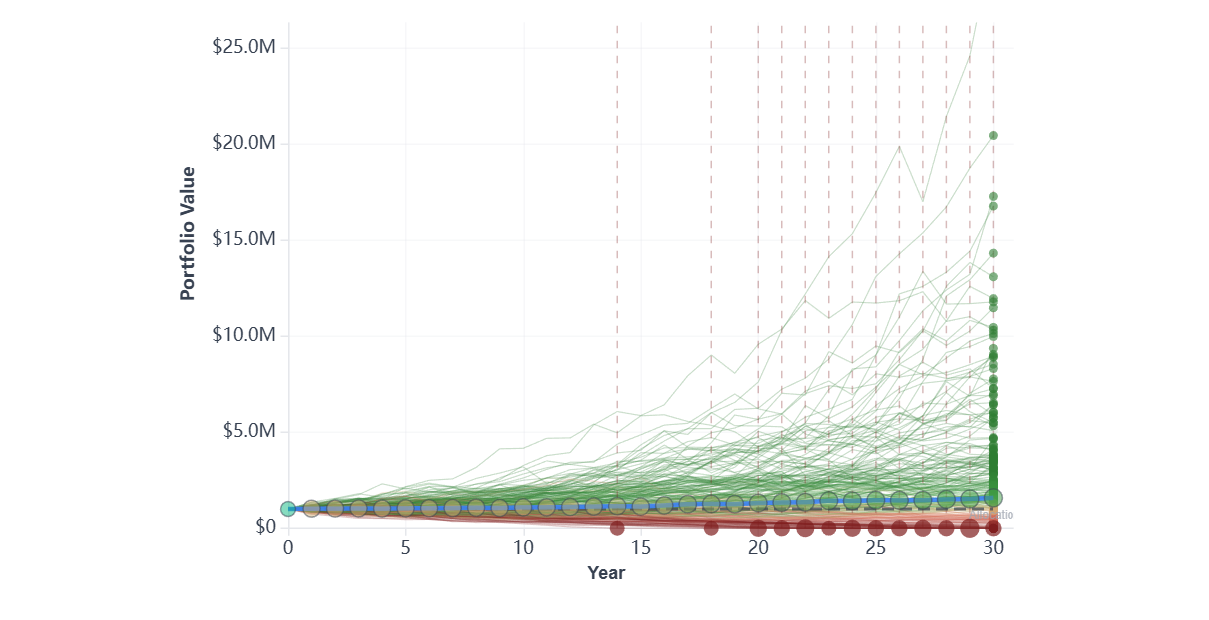
Monte Carlo: 1,000 Simulated Paths from the Same Calibration
Each thin line is one synthetic 30-year future, sampled from a normal distribution calibrated on the same Shiller history. The bold dark line is the median path; dashed lines mark the 5th and 95th percentiles. Most paths end above $1M in real terms; the lowest 5% end depleted. None of these paths actually happened — they are what the model says could happen.
This is one of many possible Monte Carlo specifications. The chart above uses correlated normal returns calibrated on the same Shiller history. Real-world Monte Carlo implementations differ substantially in their assumptions: some use Student-t or empirical distributions to capture fat tails, others use block bootstrapping or regime-switching models (Hamilton 1989) to preserve autocorrelation and momentum, others again add stochastic volatility (GARCH-style) or assume mean reversion in equity returns. Different choices produce materially different success rates on the same plan. The divergence between historical and Monte Carlo shown in Figure 3 is therefore an artefact of this particular MC model — a richer specification can shrink the gap or widen it.
Where They Agree and Where They Disagree
Distribution of final real portfolio values. The historical cohorts (green) cluster around discrete outcomes anchored to real events (the 1980s bull market, the 1966 stagflation, etc.). The Monte Carlo paths (blue) form a smoother distribution that includes outcomes history never produced — both at the high end and in the failure region. The historical success rate (~91%) and the MC success rate (~87%) are both correct answers to different questions about the same plan.
See Both Side by Side
Bellavia's historical simulation engine currently runs your plan against every actual 30-year cohort since 1871 — the green-or-red-bars view in Figure 1. Monte Carlo support is on the roadmap; when it ships, the same dashboard will show both numbers side by side, so you can spot where they agree and where the model assumptions matter.
Frequently Asked Questions
Is a 90% Monte Carlo success rate the same as a 90% historical success rate?
No. A historical 90% is a count: 9 out of 10 real periods you tested ended with money remaining. A Monte Carlo 90% is an inference: the model says there's a 90% probability your portfolio survives under its calibrated distribution. Both produce a number between 0 and 100, but they answer different questions. The worked example in this article shows the same plan giving roughly 91% historical and 87% Monte Carlo — a real gap on identical inputs.
Why do my Monte Carlo and historical results differ for the same plan?
Because they sample from different things. Historical simulation runs your plan against every actual 30-year period since 1871 — a finite enumeration of real outcomes. Monte Carlo samples from a calibrated probability distribution that includes scenarios history never produced, both at the high tail and in the failure region. Even when the Monte Carlo model is perfectly calibrated on the historical data, the historical answer is just a limited number of realizations of that distribution; Monte Carlo has more paths and explores more outcomes.
Which method is more reliable, historical or Monte Carlo?
Neither is universally more reliable; they answer different questions. Historical tells you whether your plan would have survived every real market environment on record — including 1929, the 1970s stagflation, and 2008. Monte Carlo tells you the probability of survival under a statistical model of returns, which extends coverage beyond history but carries model assumptions. When both methods say your plan works, you have stronger confidence; when they disagree, the gap is informative — it shows where the model diverges from observed history.
Does historical backtesting give a "safe" withdrawal rate?
It gives a withdrawal rate that survived all or most historical 30-year periods on the dataset you use. Whether that rate is safe in the future depends on whether future markets resemble past ones. Pfau (2010) tested the U.S. 4% rule across 17 developed-country histories and found "safety" in only 4 — meaning the historical answer is highly sensitive to which history you sample. The U.S. enjoyed an unusually favourable 20th century, so U.S. historical SWRs may be optimistic.
If overlapping periods make historical simulation statistically flawed, why use it?
Because historical simulation isn't statistical inference. The 1929 retiree and the 1930 retiree share 29 years of data, which is fine because you're not estimating a probability — you're checking whether your plan would have survived each actual starting year. The overlap critique applies when you're trying to recover a population parameter from a sample. When you're enumerating real scenarios as stress tests, overlapping periods are a feature, not a flaw.
References & Sources
- Hamilton, J.D. (1989). "A New Approach to the Economic Analysis of Nonstationary Time Series and the Business Cycle." Econometrica, 57(2), 357–384.
- Bengen, W.P. (1994). "Determining Withdrawal Rates Using Historical Data." Journal of Financial Planning, 7(4), 171–180.
- Cooley, P.L., Hubbard, C.M., & Walz, D.T. (1998). "Retirement Savings: Choosing a Withdrawal Rate That Is Sustainable." AAII Journal, XX(2).
- Pfau, W.D. (2010). "An International Perspective on Safe Withdrawal Rates from Retirement Savings: The Demise of the 4 Percent Rule?" Journal of Financial Planning, December 2010.
- Tharp, D. (2017). "Fat Tails In Monte Carlo Analysis vs Safe Withdrawal Rates." Kitces.com.
- Tharp, D. & Fitzpatrick, J. (2023). "Assessing Performance Predictiveness Of Monte Carlo Models." Kitces.com.
For the full comparison including the research on model accuracy, read: Monte Carlo vs Historical Simulation: What's the Difference?
Continue reading
- Monte Carlo vs Historical Simulation: Why They Disagree and Why That's Fine
- The Ultimate Guide to Historical Market Data for Financial Planning
- Historical Backtesting vs Monte Carlo in Retirement Planning
- How to Use Shiller Data (ie_data.csv) for Retirement Backtesting
- How to Upload JST Macrohistory Data to Bellavia
- Retirement Calculator: Inputs That Determine Success
- Sequence of Returns Risk: Why Retirement Timing Can Make or Break Your $1M Portfolio
Discussion (0)
Join the conversation
Log in to commentNo comments yet. Be the first to share your thoughts!