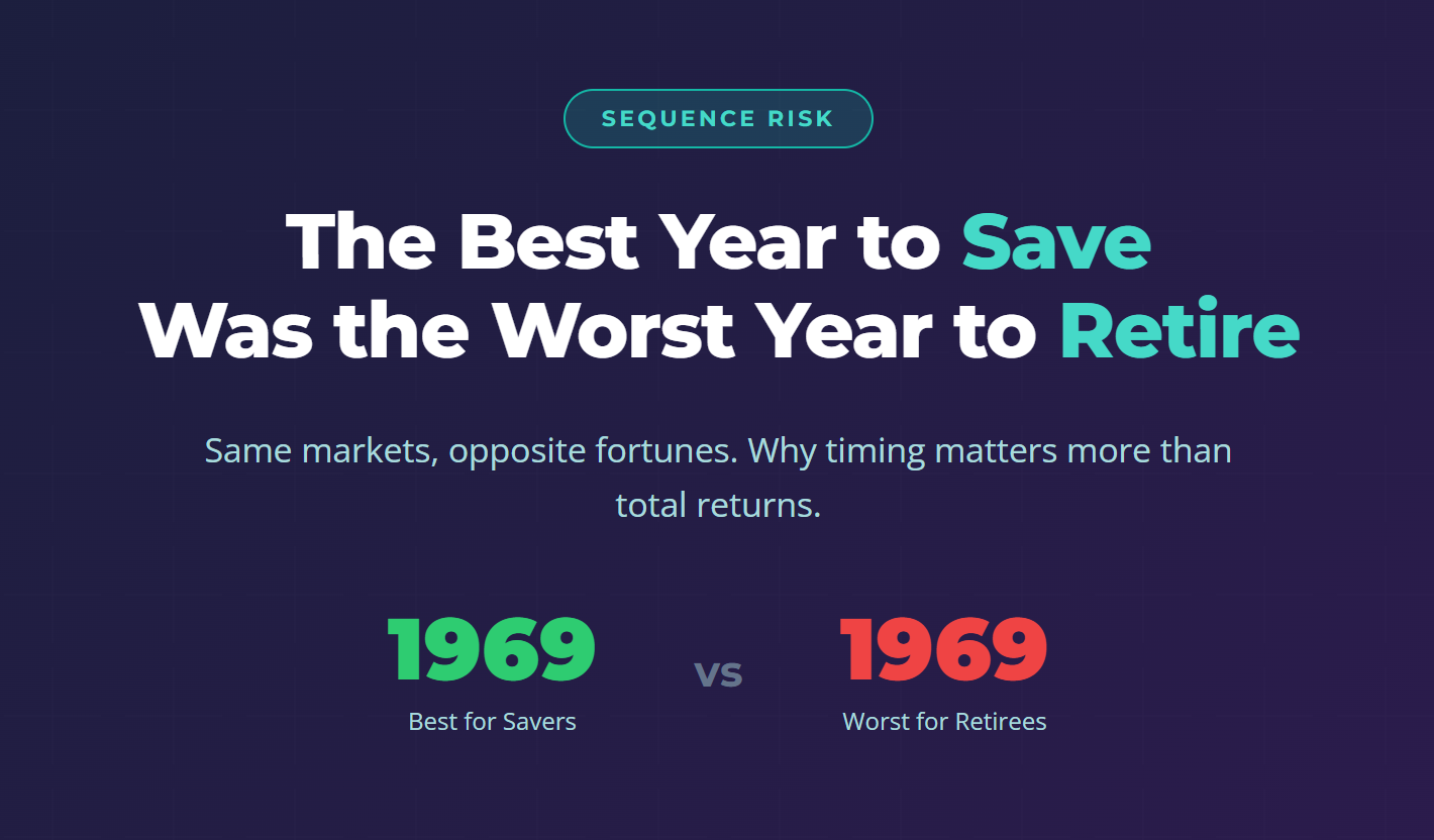
Introduction
The conventional wisdom is that markets are good or bad. But the reality is more nuanced. Whether markets help or hurt you depends entirely on where you are in your financial life. In this post, I will take up again the question of sequence of returns that was so important when discussing the savings formula. To illustrate what is happening we'll follow four people through two overlapping 30-year periods. Let's call them Saver 1, Retiree 1, active between 1949 and 1979, and Saver 2, Retiree 2, active between 1969 and 1999.
The Setup
The two 30-year historical periods we will be looking at are 1949-1979 and 1969-1999. As will be obvious, the choices is not accidental. For each period, we will consider someone who just started their savings journey and someone who just started their retirement journey. To make the saver and retiree journeys somewhat comparable, we will assume that both Saver 1 and Saver 2 save $30,000/year for 30 years following the 3% rule for savings that should practically guarantee them $1,000,000 of savings. Meanwhile, Retiree 1 and Retiree 2 both start with $1,000,000 and draw $40,000 per year following the 4% retirement rule. We will also assume all of them invest their portfolio 60% in US equity, S&P 500, and 40% in US government bonds. We will use Shiller's dataset for the following calculations.
The Historical Context
The timeframe of interest covering both 30-year periods stretches from 1949 to 1999. The two periods have a 10-year overlap from 1969 to 1979. Here is how S&P 500 performed during this period in nominal terms.
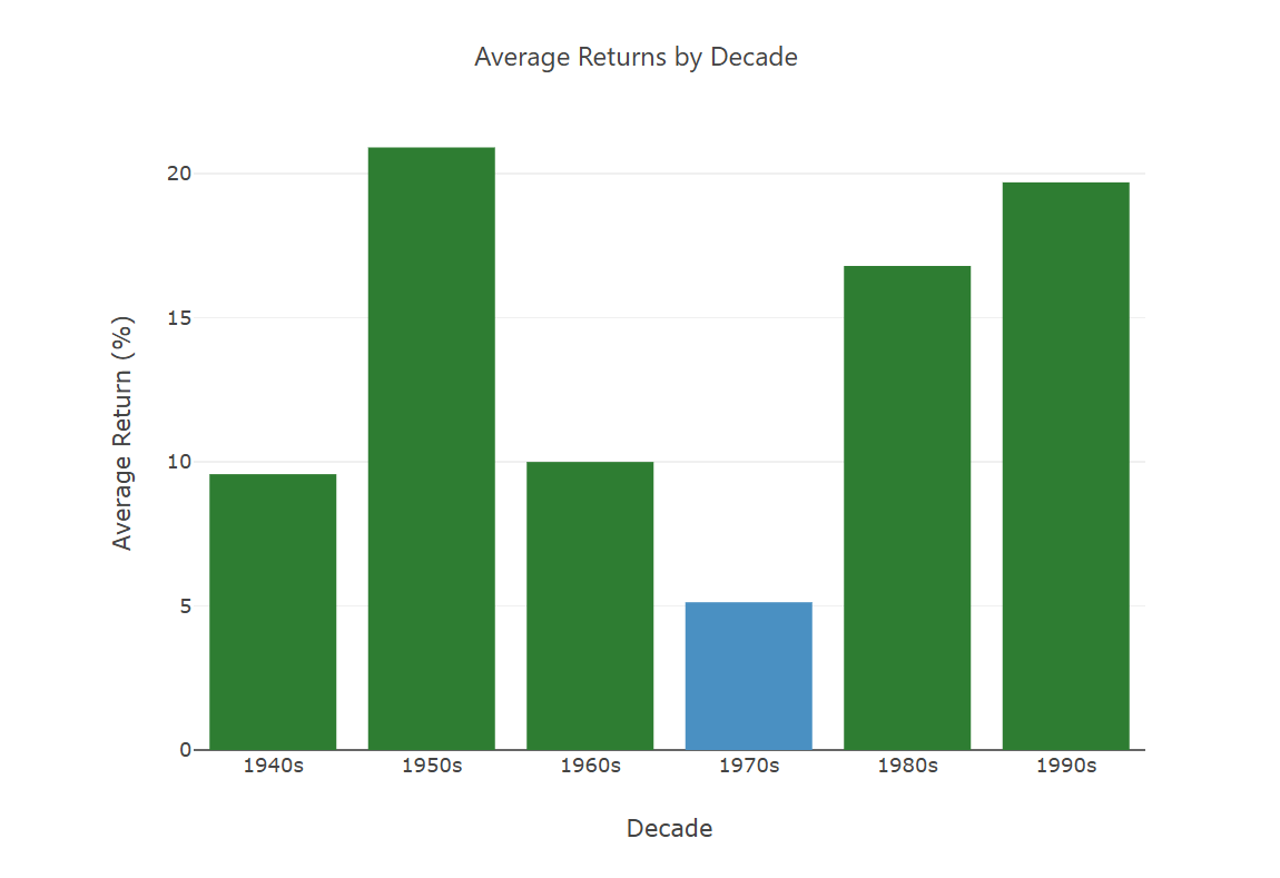
We observe that in nominal terms the market had a positive average return in each of these decades. However, we can't ignore inflation and this is what it looked like over the same period.
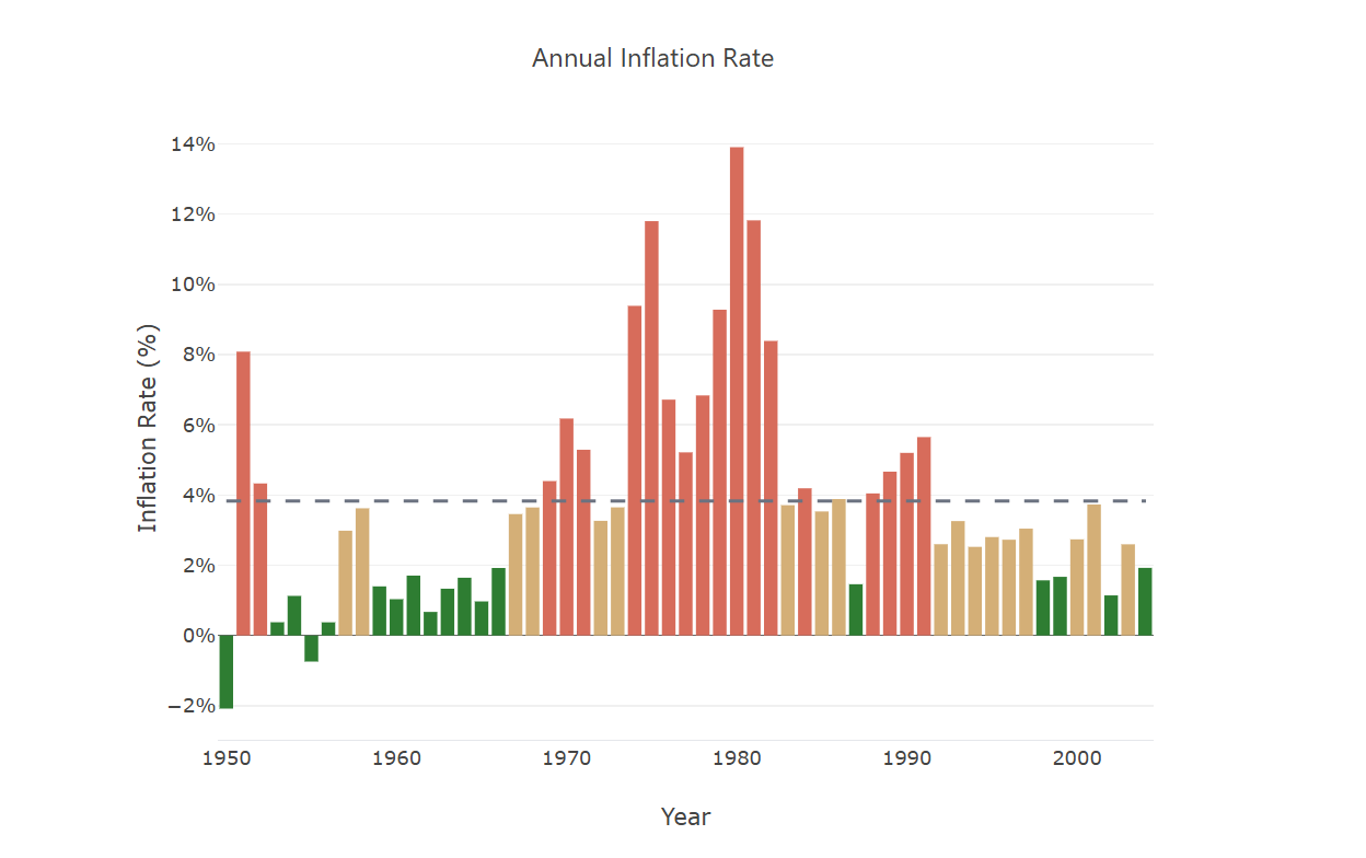
What we see in the above figure is that inflation in the 1970s and early 1980s was high, reaching 14% in 1980. As we are only interested in real returns, we have to factor this in. In the following chart we see the average real return of S&P 500 per decade.
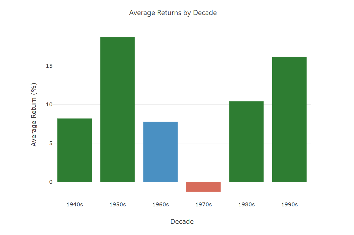
What we observe then is that the real return in the 1970s was negative: -1.27%. This was a period of stagflation, oil shocks, and the end of Bretton Woods. So, overall, we have the following picture for real returns: very high in the 1950s and 1990s, lower but positive in the 1960s and 1980s and negative in the 1970s. So, the pattern in these decades is: high - moderate - low - moderate -high. Overall, the real return from 1949 to 1979 and again from 1969 to 1999 was very close to 7% on a CAGR basis. In other words, we have two 30-year periods, overlapping with the same overall Equity market performance but with different sequences of returns. For the first period we have a sequence of returns: very positive, positive, negative per decade. For the second period the sequence of returns is inverted: negative, positive and very positive. The overall return was practically the same. So, this is an almost ideal setup to investigate actual sequence of returns for the 4 people, Saver 1, Retiree 1 and Saver 2, Retiree 2. I say almost because this test portfolio also contains 40% bonds and the bond performance which was small negative in the 50s, 60s and 70s while in the 80s and 90s was on average about 6.75%. This complicates the picture somewhat but doesn't change the conclusions.
Portfolio Performances
These are the portfolio performances given the above assumptions.
For Saver 1 who started their 30-year saving journey in 1949 saving $2,500 a month:
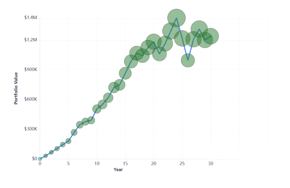
They ended up saving $1.24 Million. Given the 3% rule for savings, reaching $1M+ is to be expected. If you save 3% of the target amount then history says that there are very high chances of meeting your savings goal. The first 20 years went very well, but the poor performance of the 70s has limited their upside.
In the meantime, how did Retiree 1 do over the same years?
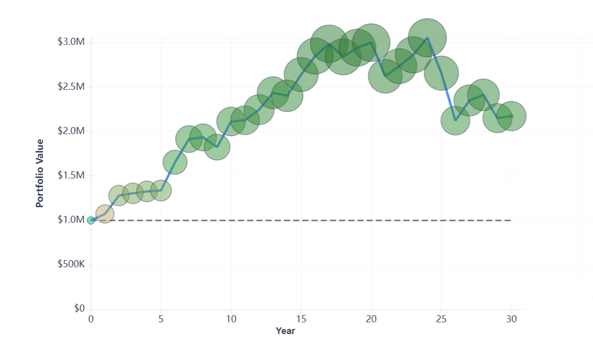
Not only were they able to draw $40,000 per year, following the 4% rule, but they were left with $2.17M after 30 years of withdrawals! Indeed, they could have drawn twice as much per year and their portfolio would still hold up.
Moving to the next period, we can look at Saver 2 who started saving in 1969. They saved $30,000 per year following the "3% rule".
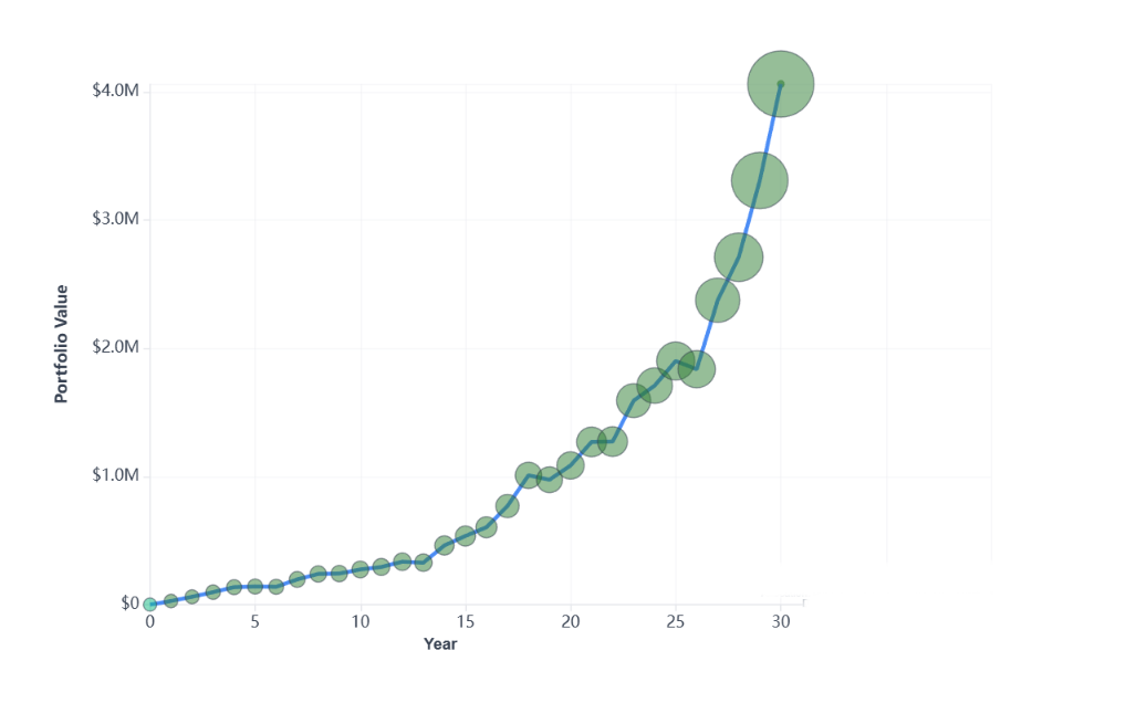
They did exceptionally well, ending up with $4 Million in 1999! If their goal was $1,000,000 they could have achieved it by saving just $7,500 per year or $625 per month!
Finally, Retiree 2, that started his retirement in 1969:
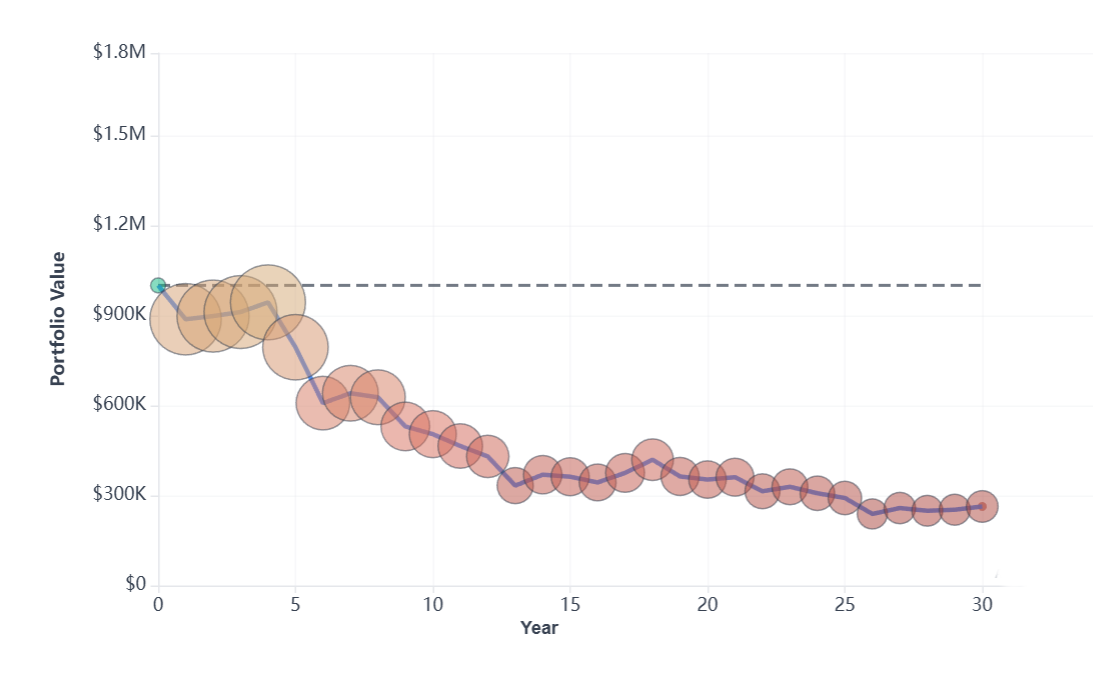
They did make it, they managed to draw $40,000 per year for a 30-year period as planned. After all, this is why the 4% rule exists, it is historically robust. However, at the end of their retirement they had just $263K left in their portfolio. This is a far cry from the $2.17M that Retiree 1 had left!
This is how the above situation can be summarized. This is what the market did:
| Decade | S&P 500 Real Return | Gov Bond Real Return | Inflation |
|---|---|---|---|
| 1950s | 18.71% | -0.45% | 1.95% |
| 1960s | 7.80% | 0.88% | 2.08% |
| 1970s | -1.27% | -1.22% | 6.76% |
| 1980s | 10.42% | 6.91% | 5.96% |
| 1990s | 16.18% | 7.52% | 3.11% |
And these are the portfolio values at the end of the 30-year periods:
| Period | Saver Outcome | Retiree Outcome |
|---|---|---|
| 1949-1979 | $1.24M (disappointing) | $2.17M (thriving) |
| 1969-1999 | $4M (exceptional) | $0.26M (barely made it) |
Between 1949 and 1979, the savers did poorly and the retirees exceptionally and the other way round between 1969 and 1999.
Sequence risk for the saver and the retiree
During saving (the accumulation phase) bad early returns only apply to the already saved amount, which is a fraction of the total amount that will be deposited in the account over a lifetime. If, for example, the first month you save $1,000 and the market falls by 50% you have only lost $500. On the contrary, if the last month before retirement the market falls by 50%, you lose half your retirement fund.
During retirement (the decumulation phase) the opposite happens. Bad early returns are depleting your full capital. Given that you will be spending part of this capital anyway, as time passes it becomes harder to recover from a significant early loss.
Here we look at the two phases accumulation and decumulation as separate and we see how each is affected by the sequence of market returns. Most people will go through both phases one way or another. They will first save and then spend. Given what we said above, it follows that the worst time to retire is just after a market crash that has decimated your savings. If you start drawing from your portfolio at its lowest point, the chances of recovery are diminishing even if the market eventually turns.
It is already clear to most people that one should be flexible about spending in retirement to get the most out of their portfolio. However, another type of flexibility is also significant here which is flexibility in the timing of retirement.
What This Means for You
Most sequence risk discussions focus just on retirement. In Bellavia, we like to think of both sides of the retirement time. Also, most of the discussions tend to focus on spending flexibility in retirement. This flexibility is very important. But there's another lever: timing flexibility. If you're approaching retirement after a major crash, delaying even 1-2 years can dramatically change your trajectory. Retiring in 1971 instead of 1969 would have completely different outcomes. Timing flexibility is underexplored in the literature. Most sequence risk discussions assume a fixed retirement date and ask how to survive it. Delaying retirement is sometimes mentioned as one option among many, but rarely examined as what it actually is: the natural hedge for a timing risk. We'll return to this in future posts.
Closing
In risk management, the most effective hedge matches the nature of the risk. Sequence risk is fundamentally a timing risk, it's not about how much the market returns in aggregate, but when those returns arrive. The natural hedge for a timing risk is a timing adjustment: flexibility in retirement timing, not just in how much you spend. This is perhaps the most fitting adjustment we can make, and it sometimes costs nothing but patience.
References & Sources
Original Retirement Research
The 4% Rule Origins - Bengen, W.P. (1994). "Determining Withdrawal Rates Using Historical Data." Journal of Financial Planning, 7(4), 171-180 - Cooley, P.L., Hubbard, C.M., & Walz, D.T. (1998). Retirement Savings: Choosing a Withdrawal Rate That Is Sustainable (Trinity Study). AAII Journal, February 1998
Accumulation Phase Research
Wade Pfau - Pfau, W.D. (2011). Safe Savings Rates: A New Approach to Retirement Planning over the Life Cycle. Journal of Financial Planning, 24(5), 42-50 - Pfau, W.D. (2012). "Capital Market Expectations, Asset Allocation, and Safe Withdrawal Rates." Journal of Financial Planning, 25(1), 36-43
Sequence of Returns Risk - Pfau, W.D. & Kitces, M.E. (2014). Reducing Retirement Risk with a Rising Equity Glide Path. Journal of Financial Planning, 27(1), 38-45 - Kitces, M.E. (2015). The Ratcheting Safe Withdrawal Rate – A More Dominant Version Of The 4% Rule?
Historical Market Data
- US Market Data: Robert Shiller's U.S. Stock Markets 1871-Present and CAPE Ratio, Yale University
- Asset Allocation Research: Vanguard (2024). Principles for Investing Success
Join Our Retirement Insights Mailing List
Get exclusive historical analysis and retirement planning insights delivered to your inbox:
- Deep dives into historical market cohorts
- Withdrawal strategy analysis and best practices
- Early access to new features and research
Free insights. Unsubscribe anytime.
Discussion (0)
Join the conversation
Log in to commentNo comments yet. Be the first to share your thoughts!