A simple question appears again and again in retirement planning:
"I have $X in savings. How much can I spend?" or "How much savings is enough to spend $Y per year?"
For simplicity, we can say X=1,000,000. We will argue that while this question sounds reasonable, it is not complete. The missing variable is time. More precisely: for how long you need this income.
This post explores an empirical fact that is often overlooked but has powerful consequences for retirement planning:
Spending capacity is not determined by wealth alone. It is a function of wealth and remaining horizon.
Once you realize this, many common rules of thumb—including the famous 4% rule starts to look incomplete too.
The Motivating Puzzle
Consider two retirees:
- Both have $1 million today.
- Both invest in the same 60/40 portfolio.
- Both face the same return uncertainty.
The only difference is:
- Retiree A is at the start of a 30-year retirement.
- Retiree B is 15 years in, with only 15 years remaining.
Should they be spending the same amount? Many tools implicitly answer yes. After all, $1M is $1M. And this follows the x% rule or any other similarly constant strategy.
But, empirically, the answer is no. And not just "a little no."
The numbers tell the story:
At $50,000/year in real spending (the "5% rule"):
-
15-year retirement: 100% historical success rate
-
30-year retirement: 76% historical success rate
Same wealth. Same spending. A 24 percentage point difference in outcomes.
At $60,000/year (6% of the portfolio) the difference is even larger:
-
15-year retirement: 99% historical success rate
-
30-year retirement: 58% historical success rate
A 41 percentage point gap. What works comfortably for one retiree fails nearly half the time for the other.
What We Measure Instead
Instead of asking for a single safe withdrawal rate, we want to ask a more precise question:
Given current wealth and remaining horizon, what constant real annual spending level can be sustained under a specified risk criterion?
We repeat this calculation across:
- a range of withdrawal amounts ($30k–$100k/year),
- a range of remaining horizons (5–50 years),
- using 150+ years of historical return paths,
- with withdrawals taken at the start of each year,
- and allowing the final year to cash out remaining wealth.
This produces not a single number but a surface, a heatmap we can visualize.
The Spending Capacity Surface
The object we are looking at is a correspondence, a mapping:
(Wealth, Time Remaining) → Sustainable Annual Spending
You can visualize it in two ways. First, as a set of curves—each line represents a different spending level, showing how success rates change with retirement duration:
Figure 1: Success rate vs. retirement duration at different withdrawal levels. The green line ($40k/year, 4%) stays near 100% across all durations. The blue line ($50k/year, 5%) drops from 100% at 15 years to 76% at 30 years. --Created with Bellavia
Notice how success rates remain high for shorter durations, then diverge dramatically as the horizon extends. The green line ($40k/year, 4%) stays near 100% across all durations—the classic "safe" withdrawal rate. But the blue line ($50k/year, 5%) drops from 100% at 15 years to 76% at 30 years. The orange and red lines ($60k–$70k) fall even faster.
A single "safe withdrawal rate" is just one line, a slice of the surface.
The Key Empirical Result
The same level of wealth supports very different spending depending on how much time is left.
For historical market paths:
- Spending capacity increases as the horizon shortens.
- The increase is not linear.
- The surface bends, flattens, and steepens depending on the actual sequence of returns.
Where the cliffs are:
| Withdrawal | Stays at 95%+ | Drops below 90% | Success rate after 30 years |
|---|---|---|---|
| $40k/year (4%) | Through 38 years | At 48 years | 99% |
| $50k/year (5%) | Through 21 years | At 26 years | 76% |
| $60k/year (6%) | Through 16 years | At 18 years | 58% |
| $70k/year (7%) | Through 13 years | At 15 years | 45% |
In plain terms:
- $1M with 30 years left is a fragile resource.
- $1M with 15 years left is a very different object.
- Treating them as equivalent is a category error.
The success "cliff" for the 5% withdrawal rate happens around 22–26 years. Before that, success rates are excellent. After that, they deteriorate rapidly. This is the nonlinearity that simple rules miss.
These cliffs are not arbitrary. They reflect transitions between different dominant risk mechanisms. Early in retirement, outcomes are driven primarily by sequence risk: poor returns combined with withdrawals can permanently damage the portfolio. Later, among paths that survive this early phase, long-run return and inflation regimes become the binding constraint.
Why This Is Not Just "Obvious"
It's easy to say:
"Of course you can spend more if you have fewer years left."
What is not obvious is:
- How much more (at 5% spending: a 24 percentage point success gap between 15 and 30 years),
- How quickly the constraint loosens (the relationship is nonlinear—success is steady, then drops sharply),
- Where the cliffs are (the thresholds where "safe" becomes "risky").
In a world of deterministic returns, spending capacity would scale smoothly with horizon, much like an annuity factor.
But real markets do not behave that way. Sequence risk, drawdowns, and inflation shocks all have an effect. The shape you see in the data is an empirical object, not a theoretical one—it emerges from actual US market history.
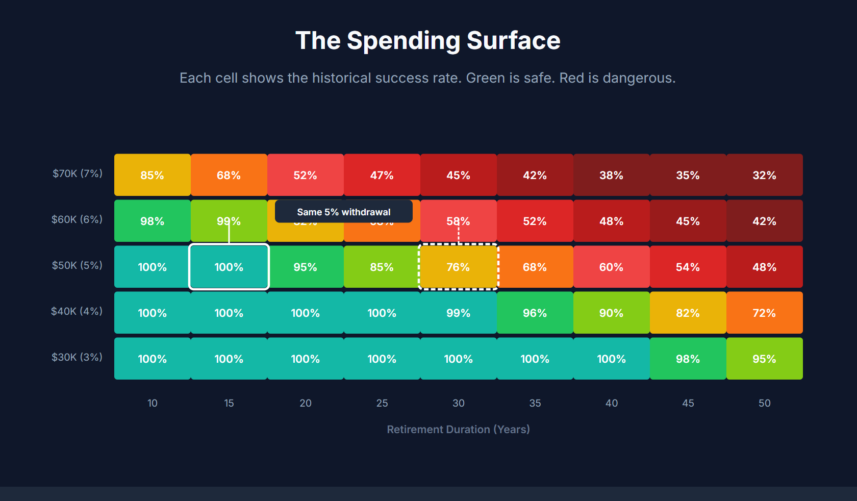
Figure 2: The spending capacity surface. Each cell shows the historical success rate for a specific withdrawal amount (y-axis) and retirement duration (x-axis). Green regions are safe; red regions are dangerous. The gradient between them reveals the terrain you're navigating. -- Created with Bellavia
All information about historical success rates for various levels of income and different horizons is encoded in this surface.
A Common Planning Mistake
Most retirement conversations implicitly collapse the problem into:
"What percentage of my portfolio can I spend?"
But a percentage alone hides two crucial facts:
- Time remaining is as important as wealth.
- Their interaction is nonlinear.
A 4% rule applied mechanically ignores where you are. So does a fixed dollar target detached from horizon. This is why dynamic withdrawal strategies often outperform fixed rules—they implicitly adapt to your changing position on the surface. This reframes the withdrawal problem: instead of searching for a universal rate, the task becomes understanding the geometry of feasible spending across states.
Practical Implications
This reframing has immediate consequences:
Spending rules should depend on both wealth and remaining years. A retiree at age 80 with 15 years of expected longevity can sustainably spend more than a retiree at age 60 with 35 years ahead—even if they have identical portfolios.
"Dynamic" withdrawal rules work by moving along this surface. Guardrails, VPW, and similar strategies are essentially mechanisms for adjusting spending as your position on the surface changes.
Recalculation of the safe rate is inherent to the problem. Your sustainable spending level changes every year as remaining time decreases and wealth fluctuates.
Comparing retirees purely by portfolio size is misleading. Two people with $1M are not in the same situation if one needs the money to last 20 years and the other needs 40.
Most importantly:
There is no meaningful answer to "how much can I spend?" without specifying how long the money must last.
How This Fits Into Bellavia
Bellavia treats retirement planning as a pathwise problem, not simply an average-outcome exercise.
The above chart is one of the natural objects that emerge from this perspective. It makes visible what single-number rules compress away.
Different assumptions (risk criteria, return models, portfolios) produce different such charts.
The Takeaway
Given the above, the right mental model is:
"Given what I have and how much time remains, what level of spending is structurally supportable?"
Once you start thinking this way, retirement planning stops being about following rules and starts being about understanding constraints.
And that understanding begins with seeing the above surface.
References & Sources
Original Retirement Research
The 4% Rule Origins
- Bengen, W.P. (1994). "Determining Withdrawal Rates Using Historical Data." Journal of Financial Planning, 7(4), 171-180
- Cooley, P.L., Hubbard, C.M., & Walz, D.T. (1998). Retirement Savings: Choosing a Withdrawal Rate That Is Sustainable (Trinity Study). AAII Journal, February 1998
Time Horizon and Withdrawal Rates
Wade Pfau on Safe Withdrawal Rates
- Pfau, W.D. (2016). The 4% Rule And The Search For A Safe Withdrawal Rate. Forbes
- Pfau, W.D. (2015). "Making Sense Out of Variable Spending Strategies for Retirees." Journal of Financial Planning, 28(10), 42-51
Dynamic Withdrawal Strategies
- Guyton, J.T. & Klinger, W.J. (2006). Decision Rules and Maximum Initial Withdrawal Rates. Journal of Financial Planning, 19(3), 48-58
- Kitces, M.E. (2015). The Ratcheting Safe Withdrawal Rate – A More Dominant Version Of The 4% Rule?
Sequence of Returns Risk
- Pfau, W.D. & Kitces, M.E. (2014). Reducing Retirement Risk with a Rising Equity Glide Path. Journal of Financial Planning, 27(1), 38-45
Historical Market Data
- US Market Data: Robert Shiller's U.S. Stock Markets 1871-Present and CAPE Ratio, Yale University
Bellavia Insights
Join Our Retirement Insights Mailing List
Get exclusive historical analysis and retirement planning insights delivered to your inbox:
- Deep dives into historical market cohorts
- Withdrawal strategy analysis and best practices
- Early access to new features and research
Free insights. Unsubscribe anytime.
Data notes: All calculations based on $1M initial portfolio, 60/40 stocks/bonds allocation, inflation-adjusted withdrawals, using Shiller market data (1871–2024). Success defined as portfolio lasting the full retirement duration without exhaustion.
Continue reading
- 1966: The Worst Year to Retire in 150 Years (And Three Other Crisis Cohorts)
- Flexible Retirement Date Windows: Mitigating Sequence And Cohort Risk
- what-if-revised
- When to Retire: How Market Timing Affects Your Savings
- Retirement Calculator: Inputs That Determine Success
- Historical 90% and Monte Carlo 90% Are Not the Same Number
- The 3% Rule for Savings
Discussion (0)
Join the conversation
Log in to commentNo comments yet. Be the first to share your thoughts!