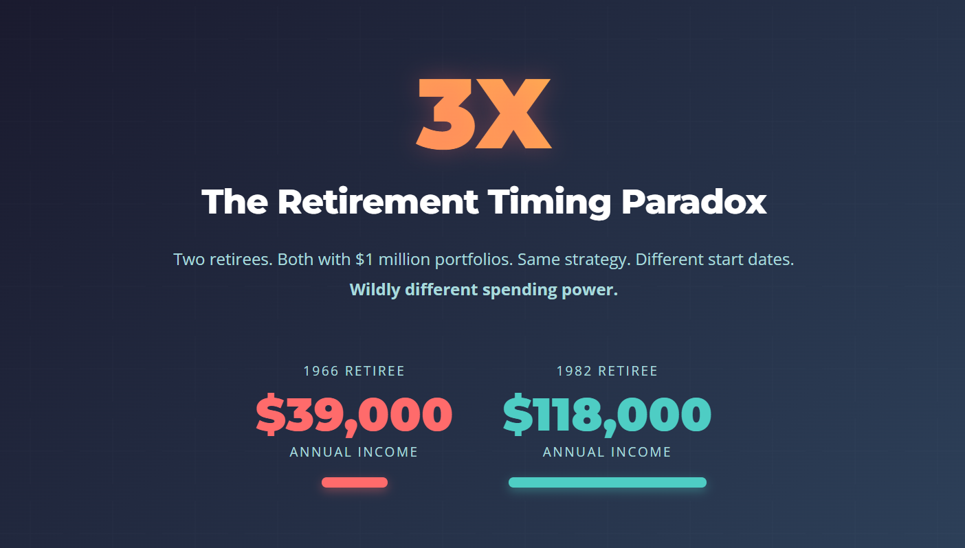
The 1966 retiree could safely withdraw only 3.9% annually (adjusting for inflation). The 1982 retiree could safely withdraw 11.8%. This is a full three times more spending power from the same starting portfolio!
This isn't just a hypothetical scenario. This is what was possible in US market history.
Building on Previous Analysis
In my recent posts on withdrawal rate failure patterns and what happens when you retire right before market crashes, I examined how different constant withdrawal rates affect portfolio longevity. Using a test portfolio, $1 million invested 60/40 in US stocks and bonds with annual rebalancing and monthly withdrawals, I traced historical patterns of portfolio degradation based on Robert Shiller's comprehensive market data.
But those analyses left one critical question unanswered:
If you could look into the future and know exactly what markets would do, what's the maximum constant withdrawal rate you could have sustained for each historical retirement period?
This isn't just academic curiosity. Understanding the range of historical outcomes—not just the worst-case scenarios—reveals crucial insights about retirement planning strategies, sequence of returns risk, and why the famous "4% rule" was designed the way it was.
The Regime View: Safe Withdrawal Rates by Historical Era
Let's start with the big picture. I've divided the past 125 years into eight distinct economic regimes, each with different market characteristics. For each regime, I calculated the safe withdrawal rate—the maximum rate that worked for every retirement cohort within that period.
What This Chart shows
The Stagflation Era (1966-1981) produced the worst conditions: A safe rate of just 3.9%. This is where the famous "4% rule" originated—from William Bengen's 1994 research examining the worst historical period.
The Great Bull Market (1982-1995) was nearly twice as generous: A safe rate of 7.6%. Retirees who happened to start in this period could sustain substantially higher spending.
Historical range spans from 3.9% to 7.6%: That's a 95% difference in sustainable spending based purely on retirement timing.
Most eras fell in the 5-7% range: The 4% rule is deliberately conservative, designed to survive even the worst period.
Why These Periods Differed So Dramatically
Stagflation (1966-1981): The Perfect Storm
- High inflation eroded purchasing power (peaking at 13.5% in 1980)
- Poor stock returns through the 1970s
- Rising interest rates crushed bond values
- Extended recovery period meant sequence risk devastated early retirees

Great Bull Market (1982-1995): Ideal Conditions
- Strong equity returns (average ~15% annually)
- Declining interest rates boosted bond returns
- Low, stable inflation
- Economic expansion across most of the period
Depression & WWII (1930-1949): Surprisingly Resilient
- Despite the Great Depression, safe rate was 4.6%
- War bonds and post-war recovery provided support
- Lower starting valuations meant better future returns
- Demonstrates that economic turmoil ≠ retirement disaster
Year-by-Year: The Granular View
Regime analysis is helpful, but it obscures variation within each period. Some individual retirement years within an era could support much higher rates than the "safe" minimum.
Here's the same analysis for every single retirement year from 1871 to 1995:
The Story the Data Tells
Massive year-to-year variation: Adjacent retirement years could differ by 1-2 percentage points in safe withdrawal rates.
Clusters of favorable periods: The 1920s, late 1940s, and 1980s-90s show consistently higher rates.
The 1960s-70s stand out dramatically: This 15-year period shows the lowest rates in 125 years of data.
Early 1900s were surprisingly challenging: The Progressive Era (1897-1906) shows rates in the 4-5% range despite economic growth.
Best single year: 1982 (11.8%): Retiring at the start of the greatest bull market in history meant you could withdraw nearly 12% annually and still survive 30 years.
Worst single year: 1966 (3.9%): Retiring right before stagflation began meant accepting the lowest withdrawal rate in recorded history.
The Combined View: Regimes and Years Together
This visualization reveals something crucial: even within challenging regimes, there's substantial variation. For example:
- Stagflation era (1966-1981): Overall, a safe rate of 3.9%, but the 1981 cohort could actually sustain 9.6%
- Depression & WWII (1930-1949): Overall, a safe rate of 4.6%, but the 1932 cohort could sustain 7.7%
This variation is why dynamic withdrawal strategies matter—adjusting your spending based on actual portfolio performance rather than blindly following a fixed rate.
Want to Test Your Strategy?
See how your retirement plan would perform across all 125 historical periods—not just the worst case.
Immediate results
What This Means for Your Retirement Planning
1. The 4% Rule Is Deliberately Conservative
The 4% rule exists because it worked in the single worst historical period (1966-1995). In the vast majority of historical scenarios, you could have withdrawn more—often substantially more.
This means:
- If you want near-certainty (surviving even the worst recorded period), 4% is appropriate
- If you're willing to adjust spending when markets underperform, higher initial rates with guardrails may work
- If you retire into favorable conditions, you might sustainably spend more than 4%
2. Your Retirement Year is Critical (but the Future Unknowable)
There is no standardized way to predict whether you'll retire into a 1966-style period or a 1982-style period. But you can:
Monitor market conditions for warning signs:
- High starting valuations (elevated P/E ratios)
- Rising inflation without corresponding wage growth
- Negative real bond yields
- Extended bull market nearing exhaustion
Use dynamic withdrawal strategies that automatically adjust based on portfolio performance. This is why guardrail approaches have gained popularity. They let you spend more in good times while protecting against depletion in bad times. We will discuss these in future posts.
Build flexibility into your retirement plan: Part-time work in early retirement, discretionary vs. essential expense categorization, and willingness to reduce spending by 10-20% if needed dramatically improve success rates.
3. Timing Risk Is Real But Manageable
These charts demonstrate why timing is so critical. Two retirees with identical portfolios but different start dates experienced vastly different outcomes. This is not because of different decisions, but because of different market timing.
Early years matter most: The 1966 retiree suffered because stagflation hit in years 1-15 of retirement. The 1982 retiree thrived because strong markets hit in years 1-13.
But it's not destiny: Even the 1966 cohort could have survived higher withdrawal rates if they'd implemented spending cuts when the portfolio dropped. The "maximum sustainable rate" assumes you never adjust, but real retirees should and do adjust.
Explore how sequence risk affects your specific plan →
Connecting to Bellavia's Analysis Tools
This historical analysis powers several of Bellavia's Premium analytical features:
Market Regimes Analysis: See which historical regime most closely resembles current conditions and what that might mean for withdrawal rates.
Sequence Risk Analysis: Understand how the timing of returns, not just average returns, determines retirement success.
Historical Simulation: Test your specific portfolio against all 125 historical periods, not just the worst-case 1966 scenario.
Test Your Plan Against History
Want to see how your specific retirement strategy would have performed in each of these 125 historical scenarios?
Test your portfolio against actual market data—including the 1966 nightmare scenario and the 1982 golden era.
Related Reading
Ready to dive deeper into historical market analysis?
- Withdrawal Rate Failure Patterns: A Historical Analysis - Understand exactly when and why retirement plans fail
- What If You Retired Right Before 1929, 1973, 2000, or 2008? - Deep dive into the worst market crashes
- The 4% Rule: Why the Creator Says His Own Formula Is Wrong - William Bengen's updated perspective
- The Value of Historical Data for Retirement Planning - Why we use actual history instead of Monte Carlo projections
Methodology & Data Sources
Analysis Parameters
- Portfolio: 60% US stocks (S&P 500), 40% US bonds
- Time Period: 1871-1995 (125 retirement cohorts)
- Retirement Duration: 30 years
- Withdrawals: Constant real (inflation-adjusted) annual amounts, taken monthly
- Success Criterion: Portfolio value > $0 after 30 years
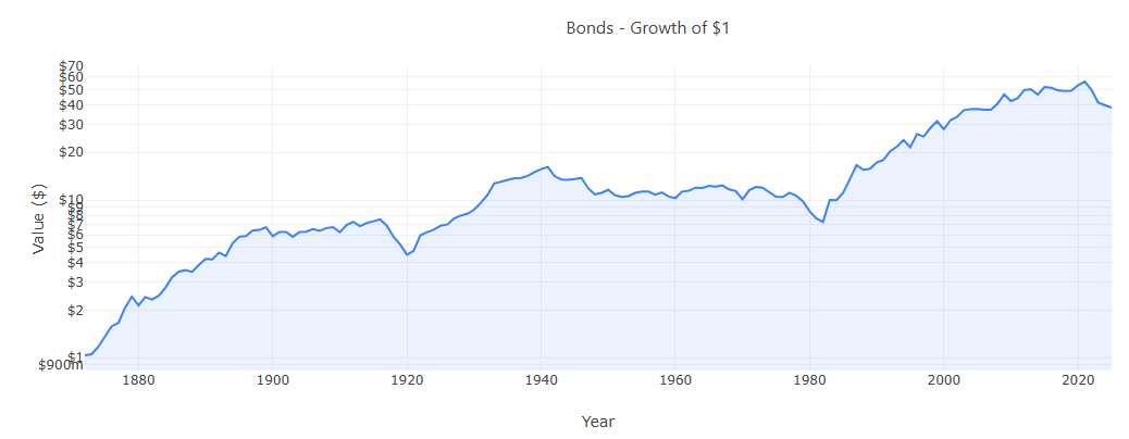
- Data Source: Robert Shiller's historical market data (1871-2025)
Definitions
Maximum Sustainable Rate: The highest inflation-adjusted withdrawal percentage that would have allowed the portfolio to last exactly 30 years, given the historical returns for that specific retirement cohort.
Safe Rate by Regime: The maximum sustainable rate within each era. This is the highest rate that worked for every retirement year in that period.
About This Analysis: All charts and calculations are based on US market data from Robert Shiller's database. Interactive visualizations created by Bellavia. Not personalized financial advice. Consult qualified professionals for investment decisions.
Questions about this analysis? Contact us
Discussion (0)
Join the conversation
Log in to commentNo comments yet. Be the first to share your thoughts!